YOLO

The “You Only Look Once” (YOLO) series of object detection models has been instrumental in advancing the field of computer vision, particularly in real-time object detection. The timeline of YOLO’s development highlights its evolution from a fast yet less precise model into a series of highly efficient and accurate tools.

Introduction of YOLO (2016)

The original YOLO model, introduced in 2016 by Joseph Redmon and collaborators, shook up the machine learning field by treating object detection as a single regression problem (Redmon et al., 2016). This innovative approach allowed YOLO to process images in one pass, resulting in excellent detection speeds. However, the initial model had limitations in accuracy, particularly with small or densely packed objects.

Interim Evolutions: 2017 to 2020

YOLOv2, released in 2017, improved on the original by adding anchor boxes, batch normalization, and a refined loss function. These changes boosted accuracy while keeping the model fast. YOLO9000, an extension of YOLOv2, could detect over 9,000 object categories, showing YOLO’s ability to handle large datasets.

YOLOv3 enhanced the model further with multi-scale detection, better handling objects of different sizes. The new Darknet-53 architecture improved feature extraction, and logistic regression enhanced accuracy, particularly for small and overlapping objects. YOLOv3 maintained a good balance between speed and accuracy, making it widely used.

YOLOv4, developed by Alexey Bochkovskiy (Bochkovskiy et al., 2020), introduced techniques like Cross Stage Partial (CSP) connections and self-adversarial training (SAT). These advancements increased both accuracy and robustness, while still prioritizing speed, reinforcing YOLO’s strong reputation.

The Newest Models: V5 and V8

YOLOv5, released in 2020 by the Ultralytics team, marked a significant shift in the YOLO series. Although not developed by the original authors, YOLOv5 quickly gained widespread adoption due to its ease of use, integration with PyTorch, and extensive documentation. It emphasized a more practical approach, optimizing the model for deployment in various real-world scenarios. YOLOv5 became a favorite among developers for its balance of simplicity, performance, and versatility, making it a go-to choice for many object detection tasks.

YOLOv8, released in 2023, represents the latest advancement in the YOLO series. It introduces cutting-edge features and enhancements in network architecture, further refining the model’s speed and accuracy. YOLOv8 is designed for seamless integration with modern hardware and software environments, making it highly adaptable and easy to deploy across a wide range of applications. This version solidifies YOLO’s position at the forefront of object detection technology, continuing the series’ tradition of innovation and excellence.

YOLO Series: Improving Speed and Precision

The YOLO series has consistently pushed the boundaries of object detection, evolving from an efficient but limited model into a series of highly sophisticated tools. YOLOv5 and YOLOv8, in particular, have become essential in real-world applications, offering unparalleled performance and ease of use. As the series continues to develop, YOLO remains a leading choice for both researchers and practitioners in the field of computer vision.

YOLOv8 In-Depth

To get insight into the function of YOLOv8, let’s look at these two picture:

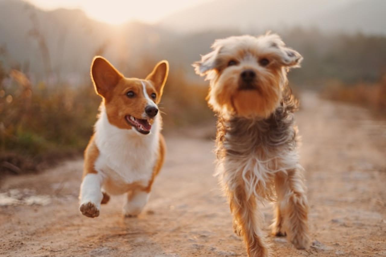
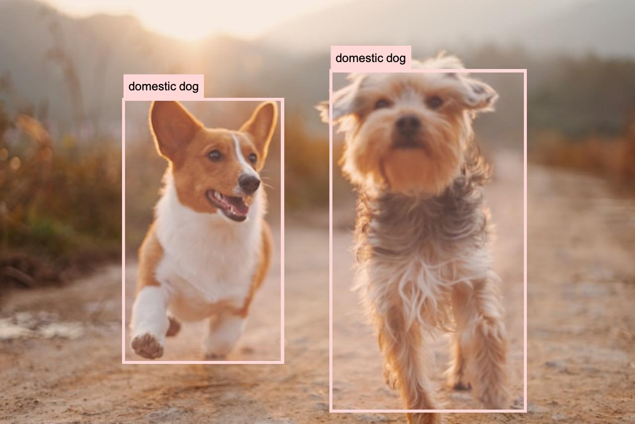
The one on the left would be the input to YOLOv8 and the right with the highlighted bounding boxes would be the output.

The function of YOLOv8 for object detection is to determine the bounding boxes for different objects in an image.

Let’s describe the three principal components of the YOLOv8 architecture using some algebra. There are the Backbone, the Neck, and Head.

Backbone

The backbone is a convolutional neural network that extracts feature maps from the input image. Let’s denote the input image as \( X \) with dimensions \( H \times W \times C \) (height \( H \), width \( W \), and \( C \) channels).

The backbone can be represented as a series of convolutional operations followed by non-linear activation functions and possibly downsampling operations (e.g., pooling or strided convolutions). Mathematically, if the backbone consists of \( L \) layers, it can be represented as:

\[F_l = \sigma(W_l \ast F_{l-1} + b_l), \quad l = 1, 2, \dots, L\]

Where:

• \( F_0 = X \) is the input image.
• \( W_l \) and \( b_l \) are the weights and biases of the \( l \)-th layer.
• \( \ast \) denotes the convolution operation.
• \( \sigma(\cdot) \) is a non-linear activation function (e.g., ReLU).
• \( F_l \) is the feature map output by the \( l \)-th layer.

The final output of the backbone, \( F_L \), is a set of feature maps \( {F_L^1, F_L^2, \dots, F_L^n} \) where each \( F_L^i \) corresponds to a feature map at different scales (e.g., multi-resolution feature maps for small, medium, and large objects).

Neck

The neck is responsible for aggregating features at different scales. This can be represented using a Feature Pyramid Network (FPN) or a Path Aggregation Network (PANet), which combine feature maps from different layers to produce refined feature maps.

For simplicity, let’s assume the neck consists of two operations: upsampling and lateral connections from the backbone. The neck can be represented as:

\[P_k = \text{Upsample}(F_{L}^k) + \text{Conv}(F_{L-1}^k), \quad k = 1, 2, \dots, n\]

Where:

• \( \text{Upsample}(\cdot) \) is an upsampling operation to match the resolution of the lower-level features.
• \( \text{Conv}(\cdot) \) represents a convolutional operation that adjusts the number of channels or refines features.
• \( P_k \) is the feature map after aggregation at scale \( k \).

The final output of the neck is a set of refined feature maps \( {P_1, P_2, \dots, P_n} \), which combine information across multiple scales.

Head

The head is responsible for generating the final predictions, including bounding boxes, objectness scores, and class probabilities. The head operates on the feature maps output by the neck.

For each scale \( k \), the head can be represented as:

\[B_k = \text{Conv}_\text{bbox}(P_k), \quad C_k = \text{Conv}_\text{class}(P_k)\]

Where:

• \( B_k \) represents the bounding box predictions for scale \( k \), including coordinates \( (x, y, w, h) \).

• \( C_k \) represents the class probabilities and objectness score predictions for scale \( k \).

• \(\text{Conv}_\text{bbox}(\cdot) \\) and \\( \text{Conv}_\text{class}(\cdot)\) are convolutional layers specific to bounding box and class prediction tasks, respectively.

The output of the head is a set of bounding boxes and associated class probabilities:

\[\text{Output} = \{(B_1, C_1), (B_2, C_2), \dots, (B_n, C_n)\}\]

Where each pair \( (B_k, C_k) \) contains the bounding boxes and class probabilities for scale \( k \).

In YOLOv8, term “scale” refers to the different levels of detail the model examines to detect both small and large objects. For example, a feature map with a resolution of \(128 \times 128\) pixels is at a different scale compared to one with \(32 \times 32\) pixels. By combining these details, it can accurately find and identify objects of various sizes in an image.

To summarize:

• Backbone: \( F_l = \sigma(W_l \ast F_{l-1} + b_l), \quad l = 1, 2, \dots, L \)

• Neck: \( P_k = \text{Upsample}(F_{L}^k) + \text{Conv}(F_{L-1}^k), \quad k = 1, 2, \dots, n \)

• Head: \(B_k = \text{Conv}_\text{bbox}(P_k), \quad C_k = \text{Conv}_\text{class}(P_k)\)

These algebraic representations provide a formal view of the operations involved in the YOLOv8 architecture, capturing the transformation of the input image through feature extraction, aggregation, and finally, object detection.

YOLOv8: Fast and Versatile

YOLOv8 is compatible with popular deep learning frameworks like PyTorch and TensorFlow. It also supports deployment on edge devices, such as Nvidia Jetson, making it versatile for various use cases:

• Surveillance systems for real-time monitoring and threat detection.
• Industrial inspection for identifying defects on assembly lines.
• Autonomous vehicles for detecting pedestrians, vehicles, and road signs.