Crafting Neural Networks

You might have visited the Neural Network Zoo (Leijnen & Veen, 2020) or looked at Wolfram Neural Net Repository and wondered how these structures came about?

Well, these layers don’t just emerge randomly. They’re crafted with precision to cater to specific requirements of various tasks, always to enhance model performance.

Convolutional Layers

For example, convolutional layers were developed to address the challenges of image processing. Digital pictures have high dimensionality and strong local relationships between pixels, which can be tricky to handle. Convolutional Layers are tailored to these characteristics, making them highly effective for analyzing images.

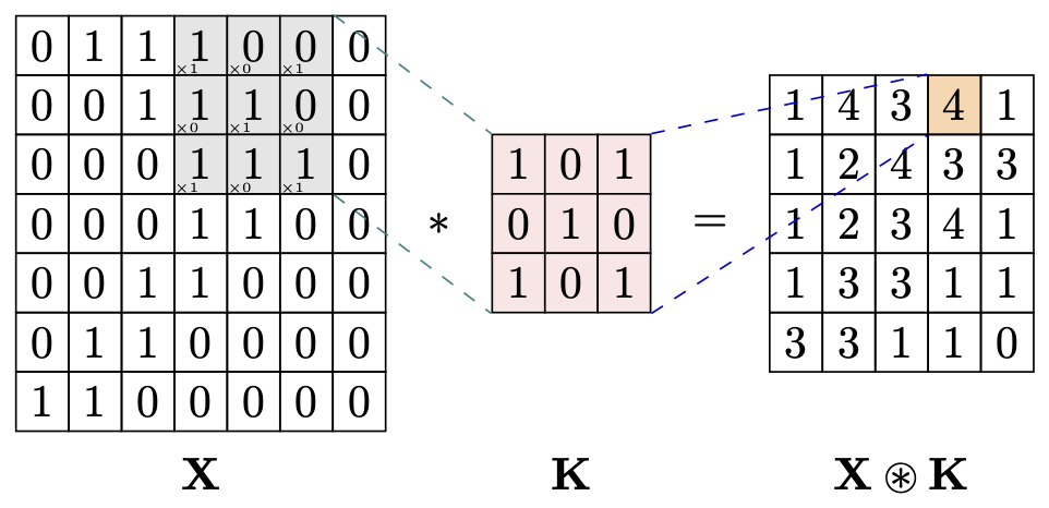
The formula for a 2D convolutional layer \(\mathbf{Y} = \mathbf{X} \circledast \mathbf{K}\) is:

\[y[i, j] = \sum_{m=0}^{M-1} \sum_{n=0}^{N-1} x[i+m, j+n] \cdot k[m, n]\]

Where:

• \( y[i, j] \) is the output feature map.
• \( x[i+m, j+n] \) is the input feature map.
• \( k[m, n] \) is the convolutional kernel (filter).
• \( b \) is the bias term.
• \( M \) and \( N \) are the dimensions of the kernel.

Note that this formula assumes no bias, no padding and a stride of 1.

New layers are usually created to overcome current limitations or to better handle specific types of data or tasks. This leads AI researchers to constantly innovate, experimenting with different layer structures, activation functions, and training methods.

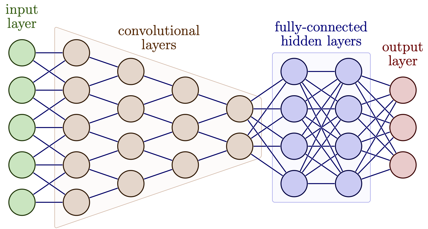
Hierarchical Feature Learning (HFL)

Another key concept in neural networks is “hierarchical feature learning,” (Krizhevsky et al., 2017) where simple features detected by early layers (like edges in an image) are combined in later layers to form more complex patterns (like shapes or objects). This hierarchy allows the model to recognize intricate patterns in the data.

HFL can be formally described using the following algebraic formulation:

Let:

• \( \mathbf{X} \in \mathbb{R}^{d_0}\) represent the input data, where \( d_0\) is the dimensionality of the input.
• \( L\) be the total number of layers in the network.
• \( \mathbf{H}^{(l)} \in \mathbb{R}^{d_l}\) represent the output (feature map) at layer \( l\), where \( d_l\) is the dimensionality of the feature space at layer \( l\).
• \( \mathbf{W}^{(l)} \in \mathbb{R}^{d_l \times d_{l-1}}\) represent the weight matrix for layer \( l\).
• \( \mathbf{b}^{(l)} \in \mathbb{R}^{d_l}\) represent the bias vector for layer \( l\).
• \( \sigma(\cdot)\) represent the activation function (e.g., ReLU, sigmoid, tanh).

The hierarchical feature encoding can be described as:

\[\mathbf{H}^{(l)} = \sigma\left(\mathbf{W}^{(l)} \mathbf{H}^{(l-1)} + \mathbf{b}^{(l)}\right), \quad \text{for } l = 1, 2, \ldots, L\]

Where:

• \( \mathbf{H}^{(0)} = \mathbf{X}\), the initial input to the network.
• \( \mathbf{H}^{(l)}\) represents the feature encoding at layer \( l\), which serves as the input to the next layer.

Low-Level Features (\( \mathbf{H}^{(1)}\)) are the basic, primitive patterns detected by the initial layers of a neural network. These features are simple and localized, including edges that mark boundaries between different regions, corners where two edges meet, repetitive textures like those found in fabric or bricks, and simple geometric shapes such as circles, triangles, or rectangles.

Mid-Level Features (\( \mathbf{H}^{(2)}, \mathbf{H}^{(3)}, \ldots\)) capture more complex patterns such as corners, contours, or parts of objects, using the low-level features as building blocks.

High-Level Features (\( \mathbf{H}^{(L)}\)) are abstract, complex patterns identified by the deeper layers of a neural network. These features often combine multiple low-level elements. Examples include recognizing specific object parts like eyes, legs, or wings, and complete objects such as a face, car, or dog. Additionally, high-level features encompass semantic concepts like identifying a “crowd of people” or “traffic scene,” as well as broader scene understanding, such as recognizing an “urban landscape” or “natural environment.”

However, designing and training deep neural networks is challenging.

Adding too many layers can lead to problems like overfitting, where the model performs well on training data but poorly on new data. Other issues, like the vanishing gradient problem, can also arise. To address these challenges, techniques like dropout layers, batch normalization, and architectures like ResNet (which uses skip connections) have been developed.

In summary, neural network layers are the result of careful research and innovation, constantly pushing the boundaries of AI. The real magic happens in how these layers learn and adapt to different tasks.